Implementing Perlin Noise and Celullar Automata to Generate Procedural 2D Maps in C++ SFML (Part 1)

Implementing Perlin Noise and Cellular Automata to Generate Procedural 2D Maps in C++ (Part 1)

Have you ever wondered how 2D rogue-like game dungeons are generated? Well, without oversimplifying the explanation, the answer can vary depending on the specific needs of the game. I'm currently exploring different rendering algorithms to create coherent maps, and while this article won't claim that all rogue-like dungeons rely on Perlin Noise and Cellular Automata, these are the two primary algorithms I’ll be explaining.

Throughout this post, we'll be implementing these algorithms in C++ and using SFML to render it in a window for visualization.

Random Vs. Procedural Generation

First we need to be able to tell the difference between randomly generated and procedurally generated maps. Even though they rely on the same principle, they differ in practice.

Procedural Generation

Procedural algorithms rely on a simple input/output (I/O) procedure. We usually recognize this approach as entirely deterministic in nature, i.e., one could predict exactly what the output would look like if one knows the input.

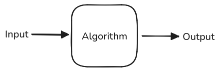
Although the above illustration is a generic representation of any algorithm, it effectively showcases the process behind procedurally generated output. Typically, the input is a 2D grid where each cell represents a pixel with a specific RGB value or a designated sprite. The algorithm's role is to assemble the map in a way that adheres to a set of pre-defined rules, ensuring it resembles a coherent layout. Of course, we could add randomness by feeding the algorithm with a random input at the start, but this is solely a matter of choice.

The resulting output is the generated map. We could iterate the process by reusing the output as new input and running it through the algorithm again.

Procedural generation, at its core, refers to creating map content based on a pre-defined set of rules — the procedure. This means that the assets of the map, whether sprites or pixel RGB values, are not pre-existing at compile time. Instead, they are generated dynamically at runtime as needed by the procedure.

Randomly Generation

Random generation involves assigning each pixel a value randomly. When we say "random," what we truly mean is "pseudo-random," as true randomness is currently unattainable in computer science. True random numbers exist only in non-deterministic systems, such as those in quantum physics. For simplicity, we’ll refer to pseudo-random numbers as random numbers moving forward.

A procedural map can appear random to the end users because they have no way of knowing how the final output will look, even though it is deterministic. However, purely random generation typically involves making decisions like determining the RGB color or sprite of a pixel without considering its surroundings. This approach lacks the structured rules that a procedural system follows. For instance, a procedural map might impose a rule that a pixel can only be either A or B. This means the selection between A and B can be made randomly, therefore this specific pixel output will in fact be unpredictably chosen from A or B. This distinction encapsulates what random generation entails.

In this article we shall mix the randomness in our procedural algorithms to make it more dynamic.

Perlin Noise

Perlin noise is a procedural algorithm widely used to generate terrains, clouds, and structured maps. Its inventor, Ken Perlin, won an Academy Award for the original implementation. While Perlin Noise can be implemented in many dimensions, we will focus on its 2D version in this article.

Perlin Noise works by dividing the 2D grid into unit squares. To compute the noise value at a specific point, we generate pseudo-random gradient vectors for the vertices (corners) of the unit square containing the point. These gradient vectors can be chosen randomly, but improved implementations, such as Improved Perlin Noise, select them from a fixed set of unit vectors to ensure consistency and eliminate directional bias.

The algorithm takes a 2D point as input, representing the x and y coordinates on the plane. These coordinates determine the specific location within the grid where the Perlin Noise function will be evaluated. You can think of the Perlin Noise grid as an infinitely large, smooth "height map" where each point has a noise value.

The output is a float value, typically within the range of [-1.0, 1.0], representing the noise value at the given coordinates. This value corresponds to the "intensity" of the noise at that location, with smooth transitions ensuring natural-looking patterns.

Unit Square Vs. Coordinate Points

We have been abstractly discussing unit squares and coordinate points, but we must now define what they represent in our implementation of the algorithm. We could think of coordinate points as individual pixels on the screen, whereas a unit square is a conceptual region of the noise grid containing multiple pixels. To accurately compute Perlin Noise, we need to calculate the noise value for each pixel in the rendered window.

Of course, this depends on the use case, so the choice of what represents what is entirely application-dependent. For our use case, it’s sufficient to assume that coordinate points correspond to pixels and that the unit square is defined arbitrarily.

Now, how is Perlin Noise actually computed? Given the corners of a unit square in the grid and their pseudo-random gradient vectors, we first calculate four additional vectors, each representing the distance from a corner to the pixel's coordinate point within the unit square. The noise value is then computed as the dot product of each corner's gradient vector and its corresponding distance vector, producing four influence values. Finally, these four values are interpolated together to yield the final noise value.

Implementation

Now that we have a solid foundation of what it Perlin Noise, let's implement it. We need five functions on total, one to sample the Perlin Noise on a given pixel coordinate x and y; another to compute the dot product of the distance vectors with their gradient counterpart; yet another one for computing simple dot product between two vectors; one cubic interpolation function; and finally a function to give us a random gradient vector given the pixel coordinates of the square corner.

#ifndef _PERLIN_NOISE_PERLIN_HPP
#define _PERLIN_NOISE_PERLIN_HPP

#include <SFML/Graphics.hpp>

// Computes dot product between two vectors
float DotProduct(sf::Vector2f vec1, sf::Vector2f vec2);

// Cubic smooth interpolation function between two floating points and 
// a weight
float Interpolate(float f1, float f2, float weight);

// Gets a random gradient vector for a square unit corner
sf::Vector2f GetRandomGradientVector();

// Computes the dot product between the unit square corner gradient
// and the distance vector
float DotGridGradient(int ix, int iy, float x, float y);

// Samples the Perlin Noise value for a given coordinate point
float SamplePerlin(float x, float y);

#endif

Now let's implement each one of these functions. Of course, we shall do it in order. The first one is the DotProduct function. For those who are not familiar with the dot product math, we simply multiply each coordinate of the first vector with its corresponding counterpart of the second vector.

float DotProduct(sf::Vector2f vec1, sf::Vector2f vec2) {
    return vec1.x * vec2.x + vec1.y + vec2.y;
}

The next one is the Interpolate function. Now, there are several interpolation functions, but we are going to implement a simple cubic smoothing interpolation function, which performs cubic smoothing interpolation. This type of interpolation creates a smooth transition between two values by easing in and easing out.

float Interpolate(float f1, float f2, float weight) {
    return (f2 - f1) * (3.0f - weight * 2.0f) * pow(weight, 2) + f1;
}

The function takes three parameters: f1 (the starting value), f2 (the ending value), and weight (a factor between 0 and 1 that determines the blend). The formula uses a cubic polynomial to adjust the weight, where the constants 3 and −2 are mathematically derived to ensure smoothness. The result is a value between f1 and f2 that changes smoothly as the weight varies.

Now let's implement the GetRandomGradientVector function. This is a simple function that should create a random vector that has its origin on the corner of the unit square grid.

sf::Vector2f GetRandomGradientVector() {
    const float PI  = 3.14159265f;
    // Uses same seed for all gradients
    static bool seedInitialized = false;
    if (!seedInitialized) {
        // Initialize a random seed
        srand(static_cast<unsigned int>(time(0)));
        seedInitilized = true;
    }

    // Get random angle
    float random = static_cast<float>(rand()) / static_cast<float>(RAND_MAX);
    random *= 2 * PI;
    sf::Vector2f gradientVector(sin(random), cos(random));
    return gradientVector;
}

To ensure the gradients are random but consistent, the function initializes a random seed using srand(static_cast<unsigned int>(time(0))). This seed initialization is controlled by a static variable, seedInitialized, which ensures the seed is only set once during the program's execution. This avoids re-initializing the seed every time the function is called, which would produce entirely new random results for subsequent pixels.

The function computes a random angle in radians, ranging from $\mathrm{}$ to $$ (a full circle). This angle is converted into a 2D unit vector using trigonometric functions: sin() for the x-component and cos() for the y-component. These calculations ensure the resulting vector is normalized, with a length of 1, and points in a random direction.

Now we implement the dot grid gradient, which should take the corner's pixel coordinate and a pixel coordinate inside the unit square as inputs and compute a random gradient vector to dot product with the distance to the pixel coordinate vector.

float GridDotProduct(int ix, int iy, float x, float y) {
    sf::Vector2f gradientVector = GetRandomGradientVector();
    sf::Vector2f distanceVector(x - (float)ix, y - (float)iy);
    return DotProduct(gradientVector, distanceVector);
}

The GridDotProduct function computes the influence of a specific corner of a unit square on a point inside that square. 

Finally, we need to sample the Perlin Noise value for a given pixel coordinate point.

float SamplePerlin(float x, float y) {
    // Determine the grid cell corner coordinates
    int x0 = (int)x;
    int y0 = (int)y;
    int x1 = x0 + 1;
    int y1 = y0 + 1;

    // Compute interpolation weights
    float sx = x - (float)x0;
    float sy = y - (float)y0;

    // Compute and interpolate top two corners
    float n0 = DotGridGradient(x0, y0, x, y);
    float n1 = DotGridGradient(x1, y0, x, y);
    float ix0 = Interpolate(n0, n1, sx);

    // Compute and interpolate bottom two corners
    n0 = DotGridGradient(x0, y1, x, y);
    n1 = DotGridGradient(x1, y1, x, y);
    float ix1 = Interpolate(n0, n1, sx);

    // Interpolate between the two previously interpolated values
    float value = Interpolate(ix0, ix1, sy);
    return value;
}

Rendering

We are now ready to render our heat map.

#include "include/perlin.hpp"
#include "include/tiles.hpp"
#include <SFML/Graphics.hpp>
#include <SFML/Graphics/RenderWindow.hpp>
#include <cmath>
#include <cstdlib>

const int WINDOW_WIDTH = 1920; // Width of the application window in pixels.
const int WINDOW_HEIGHT = 1080; // Height of the application window in pixels.
const int PIXEL_SIZE = 16; // Size of each pixel block (used for scaling grid resolution).
const int GRID_WIDTH = WINDOW_WIDTH / PIXEL_SIZE; // Number of horizontal grid cells.
const int GRID_HEIGHT = WINDOW_HEIGHT / PIXEL_SIZE; // Number of vertical grid cells.

int main() {

    // Create a render window with the specified dimensions and title.
    sf::RenderWindow window(sf::VideoMode(WINDOW_WIDTH, WINDOW_HEIGHT, 32), 
                            "Perlin Noise");

    // Allocate memory for pixel data (RGBA values for each grid cell).
    sf::Uint8 *pixels = new sf::Uint8[GRID_WIDTH * GRID_HEIGHT * 4];

    const int GRID_SIZE = 1000; // Scale of the Perlin noise grid (affects frequency).

    // Loop through each grid cell to compute and assign noise values.
    for (int x = 0; x < GRID_WIDTH; x++) {
        for (int y = 0; y < GRID_HEIGHT; y++) {
            int index = (y * GRID_WIDTH + x) * 4; // Calculate the starting index in the pixel array for this grid cell.

            float val = 0; // Initialize the Perlin noise value for this pixel.
            float freq = 1; // Starting frequency for the noise.

            // Add multiple octaves of Perlin noise for this pixel.
            for (int i = 0; i < 12; i++) { 
                val += SamplePerlin(x * freq / GRID_SIZE, y * freq / GRID_SIZE); // Sample noise at the current frequency.
                freq *= 2; // Double the frequency for the next octave.
            }

            // Adjust contrast by scaling the noise value.
            val *= 1.2f;

            // Clip the noise value to stay within the range [-1.0, 1.0].
            if (val >= 1.0f) {
                val = 1.0f;
            } else if (val < -1.0f) {
                val = -1.0f;
            }

            // Map the noise value from [-1.0, 1.0] to [0, 255] for grayscale color.
            int color = (int)(((val + 1.0f) * 0.5f) * 255);
            pixels[index] = color;       // Red channel.
            pixels[index + 1] = color;   // Green channel.
            pixels[index + 2] = color;   // Blue channel.
            pixels[index + 3] = 255;     // Alpha channel.
        }
    }

    // Create and configure an SFML texture and sprite.
    sf::Texture texture;
    sf::Sprite sprite;
    texture.create(GRID_WIDTH, GRID_HEIGHT);

    texture.update(pixels); // Upload the pixel data to the texture.
    sprite.setTexture(texture); // Set the texture to the sprite.

    // Main application loop.
    while (window.isOpen()) {
        sf::Event event;

        // Handle events (e.g., window close).
        while (window.pollEvent(event)) {
            if (event.type == sf::Event::Closed) {
                window.close();
            }
        }

        window.clear();      // Clear the window.
        window.draw(sprite); // Draw the sprite to the window.
        window.display();    // Display the updated frame.
    }

    // Clean up dynamically allocated memory.
    delete[] pixels;
    return EXIT_SUCCESS;
}

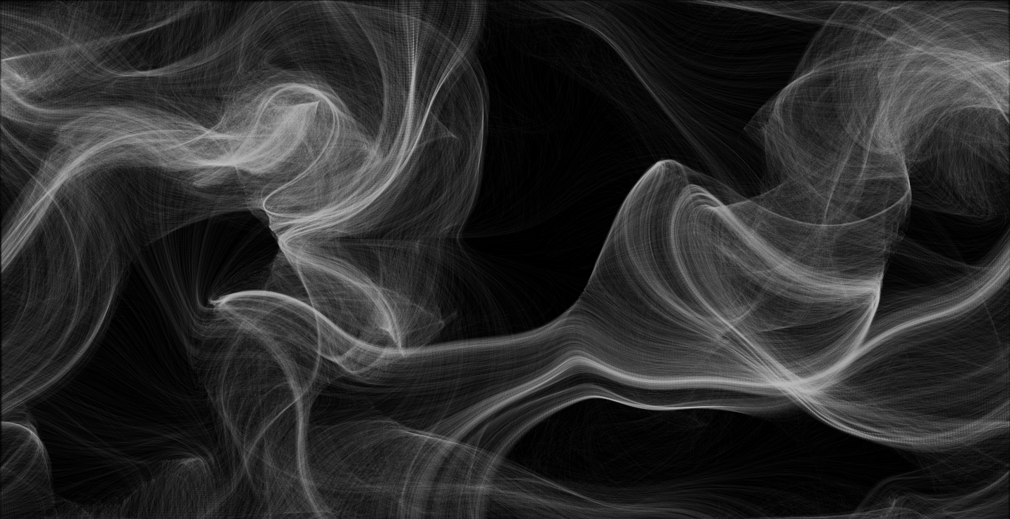
The program creates a 2D grid by dividing the window dimensions into smaller pixel blocks, where each block corresponds to a grid cell. Perlin Noise is sampled for each cell, with multiple octaves added to create finer details. The resulting noise values are scaled, adjusted for contrast, and clipped to remain within a valid range. These values are then mapped to grayscale color intensities, with higher noise values producing brighter pixels. The pixel data is stored in an array and rendered onto the screen as a texture using SFML. The final result is a visually smooth and dynamic heat map, generated procedurally in real time.

Conclusion

This article explains the implementation of Perlin Noise and how it is used to generate procedural 2D maps, such as heat maps. The program divides the screen into smaller grid cells, computes Perlin noise values for each cell, and visualizes the result in real time. Through multiple layers of noise, known as octaves, we achieve a smooth and detailed heat map, where each pixel's brightness corresponds to its noise value.

The structured approach combines randomness with predefined rules, making the output dynamic yet coherent. In the final implementation, we rendered this heat map using SFML and discussed how Perlin Noise functions work under the hood, including gradient vectors, dot products, and cubic interpolation.

As a teaser for future work, the generated grid will later serve as input for a Cellular Automata algorithm to produce natural-looking 2D caves. Stay tuned for the next article where we explore this exciting addition!